What are Vision Transformers?
2022 became the year of artificial intelligence, with incredible developments in AI art, natural language processing, computer vision, and audio technologies. Both Hugging Face and OpenAI made waves in the field. Compared to previous years, these AI technologies became more democratized and reached end users more effectively.
Today, I’ll discuss one of these developments: Vision Transformers. The article progressively deepens and becomes more technical, so I’ve structured the flow from simple to complex. You can go as far as your interest in this topic takes you.
While writing this article, I drew from many sources, blogs, my own knowledge, and even ChatGPT. If you want to do deeper reading, please check out the sources section!
TL; DR
In 2022, Vision Transformer (ViT) emerged as a competitive alternative to convolutional neural networks (CNNs), which are currently state-of-the-art in computer vision and therefore widely used in different image recognition tasks.
ViT models perform nearly 4 times better than the current state-of-the-art (CNN) in terms of computational efficiency and accuracy.
This article will cover the following topics:
- What is Vision Transformer (ViT)?
- Vision Transformers vs Convolutional Neural Networks
- Attention Mechanism
- ViT Implementations
- ViT Architecture
- Usage and Applications of Vision Transformers
Vision Transformers
For many years, CNN algorithms were virtually our only solution for image processing tasks. Architectures like ResNet, EfficientNet, Inception, etc., all fundamentally used CNN architectures to help us solve image processing problems. Today, we’ll examine ViTs (Vision Transformers), a different approach to image processing.
Actually, the Transformer concept was introduced for technologies in the NLP field. The paper published as Attention Is All You Need brought revolutionary solutions for solving NLP problems, and Transformer-based architectures have now become standard for NLP tasks.
It didn’t take long for this architecture used in natural language to be adapted to the vision domain with minor modifications. You can read about this work in the paper linked as An image is worth 16x16 words.
I’ll explain in more detail below, but the process is fundamentally based on dividing an image into 16x16 sized patches and extracting their embeddings. It’s quite difficult to explain these mechanics without covering some basic concepts, so let’s move on to the subsections to better understand the topic without losing momentum.
ViTs vs. CNN
When we compare these two architectures, we can see that ViTs are clearly much more impressive.
Vision Transformers use fewer computational resources for training while simultaneously performing better than convolutional neural networks (CNNs).
I’ll explain in more detail below, but fundamentally, CNNs use pixel arrays, while ViT divides images into fixed-size small patches. Each patch goes through a transformer encoder to extract patch, positional, etc. embeddings (topics I’ll cover below).
Additionally, ViT models perform nearly four times better than CNNs in terms of computational efficiency and accuracy.
The self-attention layer in ViT enables information to be distributed globally across the entire image, which means when we want to recombine or create new ones, this information will also be available to us - essentially, we’re teaching the model these aspects as well.
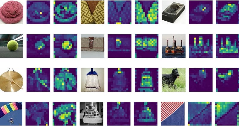 Raw images (left) with attention maps from ViT-S/16 model (right)
Source: When Vision Transformers Outperform ResNets without Pre-training or Strong Data Augmentations
Attention Mechanism
This section was written with ChatGPT
In summary, attention mechanisms developed for NLP (Natural Language Processing) are used to help artificial neural network models better process and understand input. These mechanisms work by giving different weights to different parts of the input, allowing the model to pay more attention to certain parts when processing the input.
Different types of attention mechanisms have been developed, such as dot-product attention, multi-head attention, and transformer attention. Although each of these mechanisms works slightly differently, they all operate on the principle of giving different weights to different parts of the input, allowing the model to pay more attention to certain parts.
For example, in a machine translation task, an attention mechanism can allow the model to pay attention to certain words in the source language sentence when generating the target language sentence. This helps the model produce more accurate translations because it can generate translations by considering the meaning and context of source language words.
In general, attention mechanisms are part of many state-of-the-art NLP models and have been shown to be very effective in improving the performance of these models on various tasks.
End of ChatGPT section
Since we’re focusing more on ViT in this blog, I’m going through this section somewhat quickly. For someone with no background in this area, there’s a simplified explanation beautifully presented here:
Mechanics of Seq2seq Models With Attention
ViT Implementations
Fine-tuned and pre-trained ViT models are available on Google Research’s GitHub:
You can find PyTorch implementations in lucidrains’ GitHub repository:
You can also quickly use ready-made models using timm:
Architecture
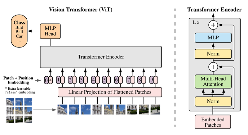
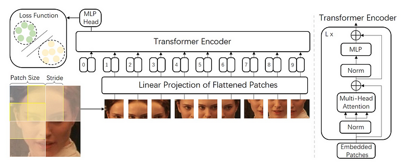
The ViT architecture consists of several stages:
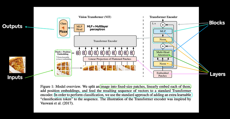
- Patch + Position Embedding (inputs):
Converts the input image into a series of image patches and adds a position number to know the order in which the patches come.
- Linear projection of flattened patches (Embedded Patches)
Image patches are converted to embeddings. The benefit of using embeddings instead of using images directly is that embeddings are a learnable representation of the image through training.
- Norm
This is an abbreviation for “Layer Normalization” or “LayerNorm”, a technique for regularizing a neural network (reducing overfitting).
- Multi-Head Attention
This is the Multi-Headed Self-Attention layer, or “MSA” for short.
- MLP (Multilayer perceptron)
You can generally think of this as any collection of feed-forward layers.
- Transformer Encoder
The Transformer Encoder is a collection of the layers listed above. There are two skip connections inside the Transformer Encoder (the “+” symbols), meaning the inputs of the layer are fed directly to the next layers as well as immediately following layers. The overall ViT architecture consists of a series of Transformer encoders stacked on top of each other.
- MLP Head
This is the output layer of the architecture, converting the learned features of an input to a class output. Since we’re working on image classification, we can also call this a “classifier head”. The MLP head structure is similar to the MLP block.
ViT Architecture
Patch Embeddings
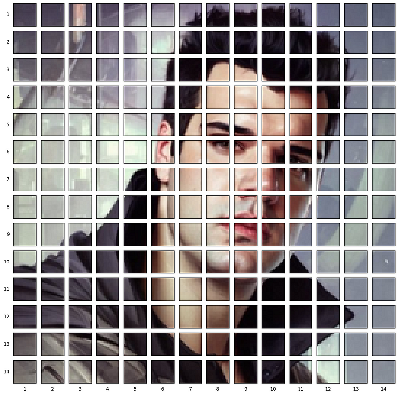
The standard Transformer takes input as a one-dimensional sequence of token embeddings. To handle 2D images, we reshape the image x∈R^{H×W×C} into flattened 2D patches.
Here, (H, W) is the resolution of the original image and (P, P) is the resolution of each image patch. The image is divided into fixed-size patches; in the image below, the patch size is taken as 16×16. So the image dimensions will be 48×48 (because there are 3 channels).
The self-attention cost is quadratic, so if we pass every pixel of the image as input, self-attention would require each pixel to attend to all other pixels. The quadratic cost of self-attention would be too high and wouldn’t scale to realistic input sizes; therefore, the image is divided into patches.
So the key point here is that dealing with individual pixels would take forever, so taking embeddings of 16x16 image patches will reduce the parameter count.
import matplotlib.pyplot as plt
from PIL import Image
import numpy as np
img = Image.open('cobanov-profile.jpg')
img.thumbnail((224, 224))
array_img = np.array(img)
array_img.shape
# Setup hyperparameters and make sure img_size and patch_size are compatible
img_size = 224
patch_size = 16
num_patches = img_size/patch_size
assert img_size % patch_size == 0, "Image size must be divisible by patch size"

print(f"Number of patches per row: {num_patches}")
print(f"Number of patches per column: {num_patches}")
print(f"Total patches: {num_patches*num_patches}")
print(f"Patch size: {patch_size} pixels x {patch_size} pixels")
# Create a series of subplots
fig, axs = plt.subplots(nrows=img_size // patch_size, # need int not float
                        ncols=img_size // patch_size,
                        figsize=(num_patches, num_patches),
                        sharex=True,
                        sharey=True)

# Loop through height and width of image
for i, patch_height in enumerate(range(0, img_size, patch_size)): # iterate through height
    for j, patch_width in enumerate(range(0, img_size, patch_size)): # iterate through width

        # Plot the permuted image patch (image_permuted -> (Height, Width, Color Channels))
        axs[i, j].imshow(array_img[patch_height:patch_height+patch_size, # iterate through height
                                   patch_width:patch_width+patch_size, # iterate through width
                                   :]) # get all color channels

        # Set up label information, remove the ticks for clarity and set labels to outside
        axs[i, j].set_ylabel(i+1,
                            rotation="horizontal",
                            horizontalalignment="right",
                            verticalalignment="center")
        axs[i, j].set_xlabel(j+1)
        axs[i, j].set_xticks([])
        axs[i, j].set_yticks([])
        axs[i, j].label_outer()

# Set a super title
plt.show()
Linear Projection of Flattened Patches
Before passing the patches to the Transformer block, the paper’s authors found it beneficial to first pass the patches through a linear projection.
They take a patch, flatten it into a large vector, and multiply it with an embedding matrix to create patch embeddings, which, combined with positional embeddings, is what goes to the transformer.
Each image patch is flattened into a 1D patch by combining all pixel channels in a patch and then linearly projecting this to the desired input dimension.
I think you’ll understand what I mean much better with this visualization:
Source: Face Transformer for Recognition
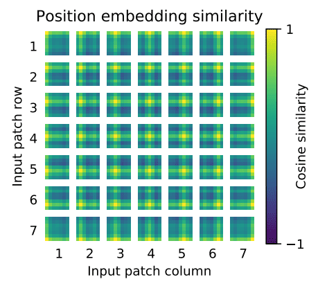
Positional Embeddings
Just as the order of words in language completely changes the meaning of the sentence you construct, we need to pay attention to this in images as well. Unfortunately, transformers don’t have any default mechanism that considers the “order” of patch embeddings.
Think of doing a jigsaw puzzle - when the pieces you have (i.e., the patch embeddings we made in previous steps) come in a mixed order, it’s quite difficult to understand what’s happening in the entire image, and this applies to transformers as well. We need a way to enable the model to infer the order or position of the puzzle pieces.
Transformers are agnostic to the structure of input elements. Adding learnable positional embeddings to each patch allows the model to learn about the structure of the image.
Positional embeddings allow us to convey this arrangement to the model. For ViT, these positional embeddings are learned vectors with the same dimensionality as the patch embeddings.
These positional embeddings are learned during training and (sometimes) during fine-tuning. During training, these embeddings converge in vector spaces where they show high similarity to neighboring positional embeddings that share the same column and row.
Transformer Encoding
- Multi-Head Self Attention Layer (MSA): used to linearly map multiple attention outputs to expected dimensions. MSA helps learn local and global dependencies in the image.
- Multi-Layer Perceptrons (MLP): Classic neural network layer but using GELU Gaussian Error Linear Units as the activation function.
- Layer Norm (LN): applied before each block since it doesn’t introduce any new dependencies between training images. Helps improve training time and generalization performance. There’s a great video by Misra here. Here’s the Paper.

- Residual connections: applied after each block because they allow gradients to flow directly through the network without passing through nonlinear activations.
- For image classification, a classification head is applied using an MLP with a hidden layer during pre-training and a single linear layer for fine-tuning. While the upper layers of ViT learn global features, the lower layers learn both global and local features. This actually enables ViT to learn more general patterns.
Summary
Yes, we’ve examined quite a few terms, theories, and architectures. To better organize things in our minds, this GIF nicely summarizes how the process works:

Usage
If you simply want to use a ViT, I’m including a small guide here as well.
You’ve probably encountered this - now when something new comes out in the AI field, forget about implementing it, even using it has become fashionable to reduce to a few lines of code.
Let’s see how everything I explained above can be done with a few lines of Python code.
Colab link: https://colab.research.google.com/drive/1sPafxIo6s1BBjHbl9e0b_DYGlb2AMBC3?usp=sharing
First, let’s instantiate a pretrained model.
import timm

model = timm.create_model('vit_base_patch16_224', pretrained=True)
model.eval()
Let’s load our image and complete its preprocessing. I’ll use my Twitter profile photo here.

# if you want to provide your own image
# comment out the following section in the code below,
# and you can provide a local path to the filename section.
url, filename = ("https://github.com/pytorch/hub/raw/master/images/dog.jpg", "dog.jpg")
urllib.request.urlretrieve(url, filename)
import urllib
from PIL import Image
from timm.data import resolve_data_config
from timm.data.transforms_factory import create_transform

config = resolve_data_config({}, model=model)
transform = create_transform(**config)

url, filename = ("https://pbs.twimg.com/profile_images/1594739904642154497/-7kZ3Sf3_400x400.jpg", "mert.jpg")
urllib.request.urlretrieve(url, filename)

img = Image.open(filename).convert('RGB')
tensor = transform(img).unsqueeze(0) # transform and add batch dimension
Let’s get the predictions
import torch

with torch.no_grad():
    out = model(tensor)
probabilities = torch.nn.functional.softmax(out[0], dim=0)
print(probabilities.shape)

# prints: torch.Size([1000])
Let’s look at the classes of the top 5 predictions
# Get imagenet class mappings
url, filename = ("https://raw.githubusercontent.com/pytorch/hub/master/imagenet_classes.txt", "imagenet_classes.txt")
urllib.request.urlretrieve(url, filename)

with open("imagenet_classes.txt", "r") as f:
    categories = [s.strip() for s in f.readlines()]

# Print top categories per image
top5_prob, top5_catid = torch.topk(probabilities, 5)
for i in range(top5_prob.size(0)):
    print(categories[top5_catid[i]], top5_prob[i].item())
trench coat        0.422695130109787
bulletproof vest   0.18995067477226257
suit               0.06873432546854019
sunglasses         0.02222270704805851
sunglass           0.020680639892816544
Sources
- Learn PyTorch - Replicating the ViT Paper
- Vision Transformer - The AI Summer
- Visual Transformers: A New Computer Vision Paradigm
- Vision Transformer (ViT) - Viso.ai
- When Vision Transformers Outperform ResNets
By Mert Cobanov on December 18, 2022